

Journal of Creation 29(1):6–8, April 2015
Browse our latest digital issue Subscribe
A preliminary age calibration for the post-glacial-maximum period
In the past 20 years a number of studies have been published on the rise in global sea level since the last glacial maximum. The dates of the last glacial maximum and the change of sea level with time were based on long-age dating assumptions using a variety of methods, and fitted into the uniformitarian timeline.1 Given that the glacial maximum occurred toward the end of the post-Flood Ice Age, these curves allow us to develop an age calibration to convert secular, long-age dates into dates within biblical history.
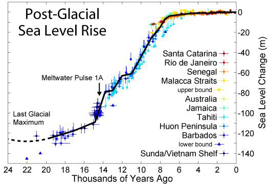
Figure 1 shows the current secular view on sea-level rise since the end of the last glacial maximum. This graph was prepared by Robert Rohde from several published papers2 that included data assembled from numerous other sources. The actual sea levels had been adjusted for vertical geologic motions such as continental rebound, connected with the removal of continental ice, and hydrostatic rebound, due to the increased weight of water in coastal areas. However, it is the dates on the chart rather than the sea levels that are primarily needed for an age calibration.
Developing the calibration curve

An analysis of the magnitude of the sea-level fall needs to be evaluated, but this is outside the scope of this article. The graph shows the last glacial maximum occurring at 22,000 years ago, when sea level was at its lowest, and the sea-level rise reaching the present level at about 7,000 years ago, all within the secular timescale.
It was the biblical Flood that provided the conditions on Earth that caused the Ice Age immediately after the Flood. The primary driver was warm oceans and a secondary factor would have been volcanic dust and aerosols high in the atmosphere.3 In his monograph on this topic Oard discusses the timing of the Ice Age, namely the time to reach glacial maximum, and the time for the ice sheets to melt back to their present size.
His ‘best estimate’ for their buildup to glacial maximum, based on a 25% depletion of solar radiation and a 12.5% decrease in the current values of the atmospheric and oceanic heat transports, is 500 years.3 From energy balance considerations he found only a short time was required for the oceans to cool, and the ice sheet to melt back. The periphery of each sheet would melt first, and quickly, and the interiors more slowly. He concluded that the best estimate for the melt-back time to present size was 200 years.3

The timing of the Ice Age is tied to the timing of the Flood, which, in round figures, can be taken as about 4,500 years ago.4 The Ice Age maximum would thus have been about 4,000 years ago and the oceans would have reached their current level about 3,800 years ago.
Hence we equate the secular date for the last glacial maximum (22 ka ago) to the biblical date of 4,000 years ago. And we tie the secular date when the oceans reached their present level (7 ka ago) to the biblical age of 3,800 years ago. The 200-year period of ice melt-back results in a very tight compression of the major part of the secular timescale. This gives us three points for our calibration curve (table 1).

We would expect the secular dates to better match historical dates (and thus biblical dates) for recent history over the last 2-3 ka, and for the calibration factor to be close to 1.0 in this range. Further, we would expect the separation between the two scales to increase with increasing age due to the effects of the Flood and the Ice Age, and thus the calibration factor would diverge more greatly from 1.0. As the secular time increased into multiple tens of thousands of years we would expect the calibration factor to become smaller and smaller, tapering off into an exponential decay type of shape. Based on this we can fit by eye a reasonable calibration curve for the period, as shown in figure 2.
From the calibration factors of figure 2 we can calculate a calibration curve as shown in figure 3, which allows us to read the biblical age for the post-glacial-maximum period when we have the uniformitarian age.
Discussion
This is a broad-brush approach to adjusting secular dates to fit in with ages based on the historical reports in the Bible. It may be claimed that the method is circular, that we have massaged the figures to get the answer that we want. This is correct, but this is the way that all dating methods work.5 All methods begins with researchers making careful measurements on samples in the present. Then they must make assumptions about the past to calculate an ‘age’. But no one stops there. All researchers compare results with other age information, and adjust assumptions and interpretations until the calculated age makes sense within its context. So, this exercise of converting secular ages to match biblical history simply follows the normal practice of geochronology, but with the great advantage that biblical history is reliable.
The carbon-14 (C14) method is the one most widely used for the period of time back to about 40,000 years ago, and so this calibration curve would reflect the sorts of adjustments that would need to be made to C14 ‘dates’ in order to obtain actual dates. The need for significant correction to C14 dates beyond a few thousand years has been long recognized even by secular geochronologists, as Pilcher discusses:
“It is most likely that at the end of the last glaciation there were considerable perturbations of the global carbon cycle with the release of old carbon from ice, and an increase in biomass as temperatures rose. … It is hard to believe that these changes would not have had dramatic effects on the radiocarbon levels in the atmosphere.”6
Secular geochronologists already have calibration curves for the C14 method to make the results agree with other methods and other information, such as dendrochronology. However, we would anticipate even larger corrections would be needed for C14 dating than those used by secular geochronologists because they ignore the dramatic effects of the Flood.
The Flood would impact many factors, including non-equilibrium levels for C14 in the atmosphere immediately after the Flood, the burial of low C14 preFlood vegetation, increased volcanism after the Flood producing ‘old carbon’ in the atmosphere, revegetation of the earth after the Flood, and changes to the earth’s magnetic field affecting C14 production in the upper atmosphere. A useful discussion of the factors affecting C14 dates as they would have been impacted by the biblical Flood and the post-Flood recovery is presented by Batten.7
Conclusion
The calibration curve (figure 3) would have general application to all dates published within the secular long-age scheme because all dating methods are compared with, and calibrated against, each other in order to obtain a consistent suite of dates. While figure 3 can be considered a general calibration curve, we would anticipate that there would be temporal and regional anomalies depending on the dating method and the study location. We will need to consult more reliable sources and obtain other information in order to refine and test the curve.

Update 16 May 2017
Following several requests by those who commented on this article, we publish here the sea level curve related to the biblical timescale (the calibration curve of figure 2 applied to data of figure 1). The sea level changes are based on the timing of the Ice Age published by Oard (ref. 3). Notice that in this figure 4, sea level rises rapidly after 4000 years ago (Ice Age Maximum) and remains very stable since. The Flood is taken at 4,500 years ago, so there would have been a similarly rapid sea-level drop after the Flood to the glacial maximum. Oard has argued that the ice sheets during the ice age were much thinner than the thickness assumed by long-age geologists. Consequently, he concludes that the sea level drop was only some 55 m rather than the 130 m shown in the diagram.
References and notes
- Yokoyama, Y., Lambeck, K., De Decker, P., Johnston, P and Fifield, L.K., Timing of the Last Glacial Maximum from observed sea-level minima, Nature 406(6797):713–716, August 2000 | doi:10.1038/35021035. Return to text.
- Rohde, R., Post-glacial sea level, Global Warming Art, globalwarmingart.com, accessed July 2014. Rohde collated information from:
(1) Fleming, K., Johnston, P., Zwartz, D., Yokoyama, Y., Lambeck, K. and Chappell, J., Refining the eustatic sea-level curve since the Last Glacial Maximum using far-and intermediate-field sites, Earth and Planetary Science Letters 163(1–4):327-342, 1998.;
(2) Fleming, K.M., Glacial Rebound and Sea-level Change Constraints on the Greenland Ice Sheet, Australian National University, PhD Thesis, 2000.
(3) Milne, G.A., Long, A.J. and Bassett, S.E., Modelling Holocene relative sea-level observations from the Caribbean and South America, Quaternary Science Reviews 24 (10–11):1183-1202, 2005. Return to text. - Oard, M.J., An Ice Age Caused by the Genesis Flood, Institute for Creation Research, El Cajon, CA, 1990. Return to text.
- Hardy, C. and Carter, R., The biblical minimum and maximum age of the earth, J. Creation 28(2):89–96, 2014, conclude that the Flood probably occurred between 2600 BC and 2300 BC. Return to text.
- Walker, T., How dating methods work, Creation 30(3):28–29, 2008; creation.com/dating-flaws. Return to text.
- Pilcher, J.R., Radiocarbon dating; in: Smart, P.L. and Frances, P.D. (Eds.), Quaternary Dating Methods—A User’s Guide, Quaternary Research Association, Technical Guide No. 4, Cambridge, pp. 16–32, 1991. Return to text.
- Batten, D. (Ed.), The Creation Answers Book, (4th edn.) Creation Book Publishers, pp. 68–73, 2012. Return to text.


Readers’ comments
Comments are automatically closed 14 days after publication.